Supreme Excel Add Regression Line To Scatter Plot
Add A Linear Regression Trendline To An Excel Scatter Plot Google Sheets Multiple X Axis Line Graph With Lines In R
Add A Linear Regression Trendline To An Excel Scatter Plot Ggplot Geom_line Multiple Lines Graph With Target Line
Add A Linear Regression Trendline To An Excel Scatter Plot Line Two X Axis
Add A Linear Regression Trendline To An Excel Scatter Plot Ggplot2 Y Axis Line Graph With Example
Add A Linear Regression Trendline To An Excel Scatter Plot Change Chart Scale Category Axis And Legend In
Add A Linear Regression Trendline To An Excel Scatter Plot Line Chart Canvasjs Normal Distribution Histogram
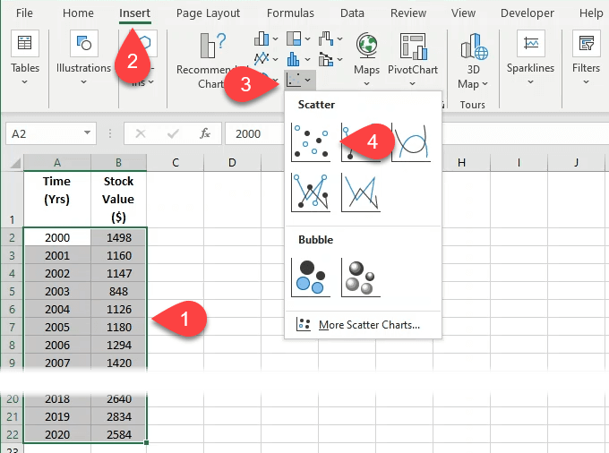
Start by selecting data in two columns.
Excel add regression line to scatter plot. Suppose you have two columns of data in Excel and you want to insert a scatter plot to examine the relationship between the two variables. Then in Excel select both columns of data by selecting and holding on the top-left number and dragging down to the bottom-most number in the right column. Introduction We continue from the earlier article Using Excel.
Add a Regression Line. Fit a simple linear regression model model. The default sub-type is what is needed for just comparing pairs of values.
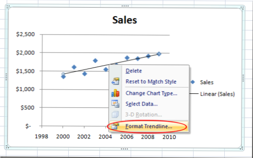
While Excel can calculate a range of descriptive and logical statistics for you it is often better to show a visual representation of the data when presenting information to a groupUsing the built-in trendline function in Excel you can add a linear regression trendline to any Excel scatter plot. Then click on the Insert tab on the Ribbon and locate. You will now see a window listing the various statistical tests that Excel can perform.
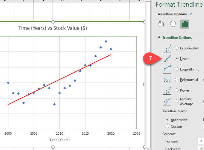
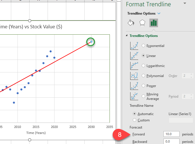
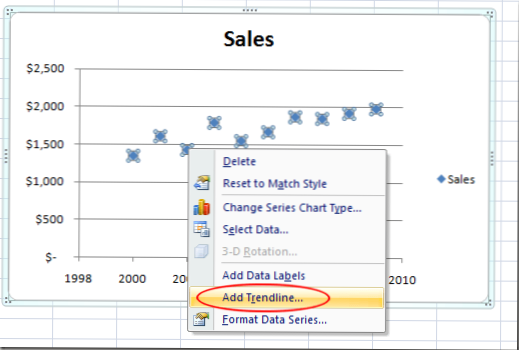
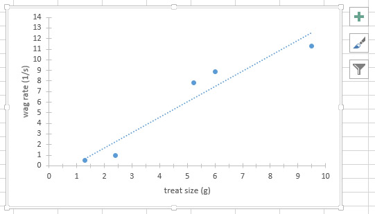
Create your scatter graph. We can do some cool things with the trendline and. Add a Linear Regression Trendline to an Excel Scatter Plot.
Inserting a Scatter Diagram into Excel. Scroll down to find the regression option and click OK. XY Scatter is the type of Chart we want.
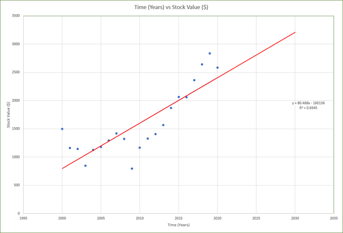
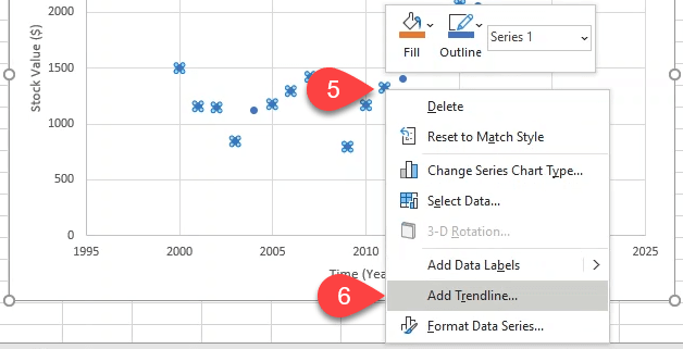
We can chart a regression in Excel by highlighting the data and charting it as a scatter plot. This will automatically add a simple linear regression line to your scatterplot. Just click add trend line and then select Logarithmic Switching to R for more power I am a bit lost as to which function should one use to generate this.

How To Add A Regression Line Scatterplot In Excel Plot Horizontal Matlab Vertical
Tambahkan Linear Regression Trendline Ke Excel Scatter Plot Tips Ms Office Kiat Komputer Dan Informasi Berguna Tentang Teknologi Modern Lines In Ggplot Three Line Break Chart

Combine Bubble And Xy Scatter Line Chart E90e50fx Data Science Excel Multi Seaborn Axis Limits
Tambahkan Linear Regression Trendline Ke Excel Scatter Plot Tips Ms Office Kiat Komputer Dan Informasi Berguna Tentang Teknologi Modern Reading Line Graphs Python Matplotlib
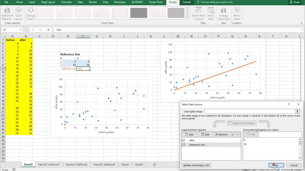
Excel Scatterplot With Reference Line Youtube Move Axis To Left Combine Two Bar Charts In
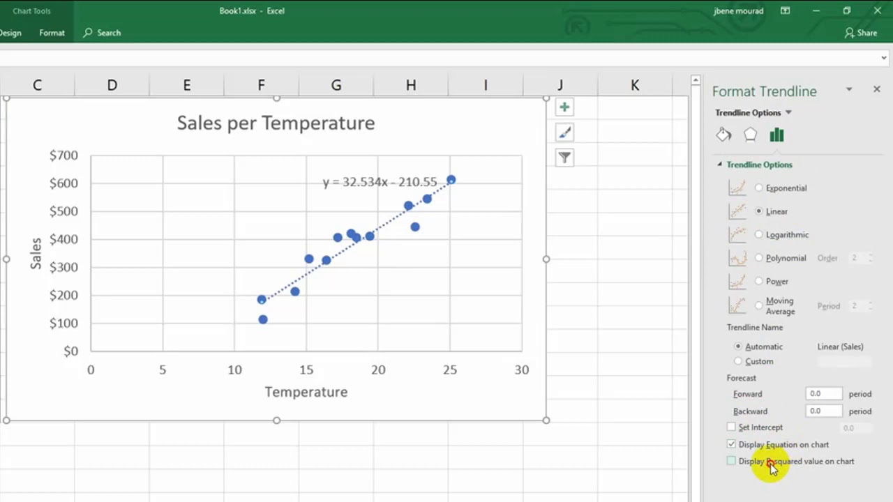
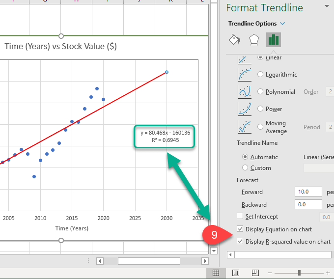
How To Make A X Y Scatter Chart In Excel Display The Trendline Equation And R2 Youtube Ggplot Vertical Line Multiple Time Series Graph
6 Scatter Plot Trendline And Linear Regression Bsci 1510l Literature Stats Guide Research Guides At Vanderbilt University Excel Date On X Axis Sas Line

How To Add Line Curve Of Best Fit Scatter Plot In Microsoft Excel Discoverbits Create Graph Free Two Lines R Ggplot2
